Intelligence
Three models that read the operation from different angles.
The models measure how efficiently each process runs and flag where it is losing ground. Operating ranges compare against normal running. The forecasting model projects operations forward. The root-cause model reconstructs backwards to find the bottleneck. Together they give you the operational picture of the plant.
01
Operating ranges
The model learns how each machine normally moves, from that machine's own history, and flags when a signal leaves that band.
It earns its keep when a value is still far from the alarm limit but has already drifted from usual. The band holds steady until it is recalibrated with more history.
02
Forecasting targets and failures
Projects forward to anticipate a target that will be missed or a failure before the signal reaches its limit. The result is a range with a confidence band around it.
The band widens with the horizon. The further out the projection, the less precise the value and the more honest it is to show a range.
03
Root cause
After an event, it traces backwards through where the problem propagated to find the origin and what to do about it.
The next morning starts with a concrete candidate to check.
What they run on
Calculated metrics derived from raw readings.
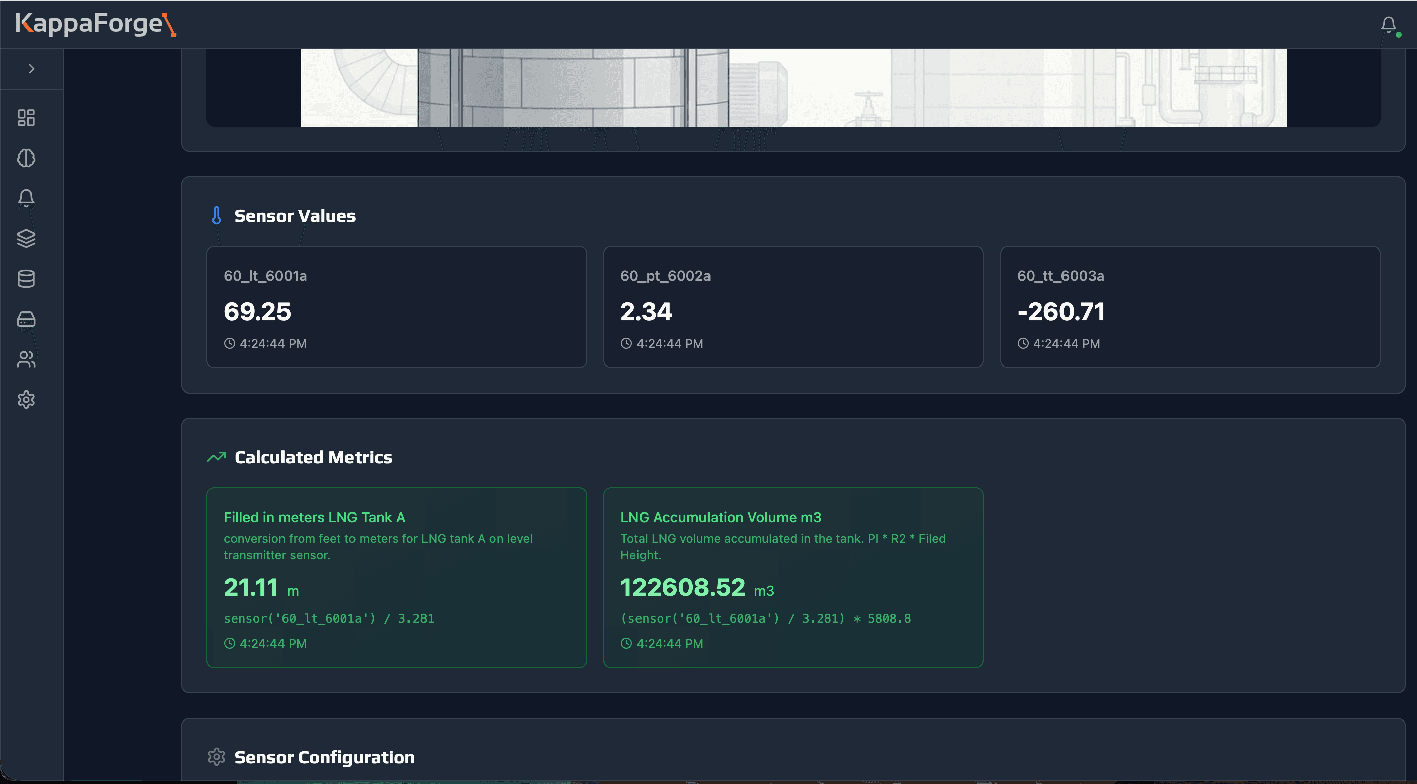
Before a model has an opinion, the sensor reading becomes the quantity the business cares about. Unit conversions, chained aggregations and multi-step calculations turn a level in millimetres into cubic metres delivered, then into a shift total, then into the monthly figure that reaches the invoice. Every metric shows the formula behind it, so the number the model works from is the same one people work from.
When they start
They begin tracking equipment on day one.
The models need history before they produce strong output, and they sharpen as that history grows. Timing follows the production cycle rather than the calendar: what matters is how many complete cycles the equipment has run.
For equipment that cycles daily, around thirty days of data is a typical starting point. A skid that works in campaigns takes longer, and we tell you where it stands rather than switching it on early.
Next step